MICROSOFT EXEL

Entering values in excel sheet is a child’s play and this chapter shows how to enter values in an excel sheet. A new sheet is displayed by default when you open an excel sheet as shown in the below screen shot.

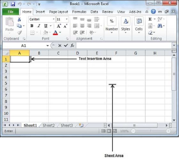
Sheet area is the place where you type your text. The flashing vertical bar is called the insertion point and it represents the location where text will appear when you type. When you click on a box then the box is highlighted. When you double click the box, the flashing vertical bar appears and you can start entering your data.

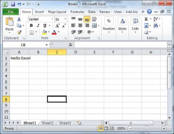
So, just keep your mouse cursor at the text insertion point and start typing whatever text you would like to type. We have typed only two words "Hello Excel" as shown below. The text appears to the left of the insertion point as you type.

There are following three important points, which would help you while typing −

• Press Tab to go to next column.
• Press Enter to go to next row.
• Press Alt + Enter to enter a new line in the same column.

Inserting Data

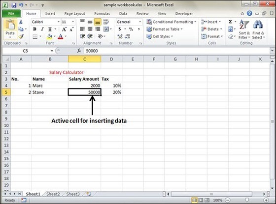
For inserting data in MS Excel, just activate the cell type text or number and press enter or Navigation keys.

Inserting Formula

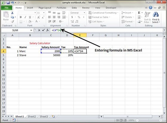
For inserting formula in MS Excel go to the formula bar, enter the formula and then press enter or navigation key. See the screen-shot below to understand it.

Modifying Cell Content

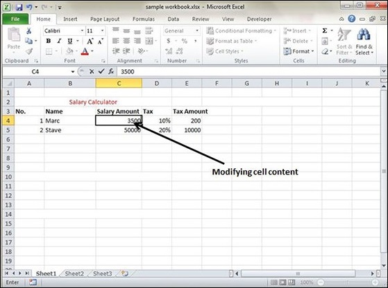
For modifying the cell content just activate the cell, enter a new value and then press enter or navigation key to see the changes. See the screen-shot below to understand it.

MOVE DATA

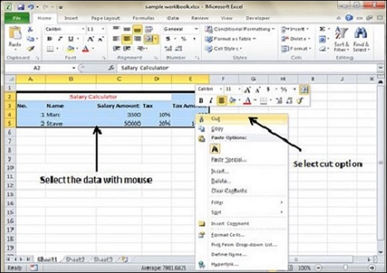
Step 1 − Select the data you want to Move. Right Click and Select the cut option.

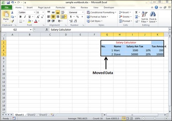
Step 2 − Select the first cell where you want to move the data. Right click on it and paste the data. You can see the data is moved now.

TEXT ALIGNMENTS

If you don’t like the default alignment of the cell, you can make changes in the alignment of the cell. Below are the various ways of doing it.

Change Alignment from Home Tab

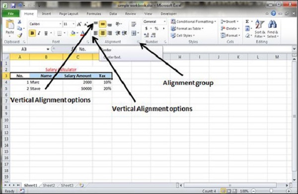
You can change the Horizontal and vertical alignment of the cell. By default, Excel aligns numbers to the right and text to the left. Click on the available option in the Alignment group in Home tab to change alignment.

Change Alignment from Format Cells

Right click on the cell and choose format cell. In format cells dialogue, choose Alignment Tab. Select the available options from the Vertical alignment and Horizontal alignment options.

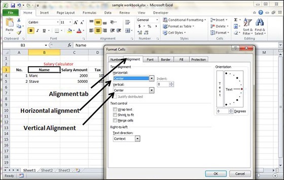
Exploring Alignment Options

1. Horizontal Alignment − You can set horizontal alignment to Left, Centre, Right, etc.

• Left − Aligns the cell contents to the left side of the cell.
• Center − Centers the cell contents in the cell.
• Right − Aligns the cell contents to the right side of the cell.
• Fill − Repeats the contents of the cell until the cell’s width is filled.
• Justify − Justifies the text to the left and right of the cell. This option is applicable only if the cell is formatted as wrapped text and uses more than one line.

2. Vertical Alignment − You can set Vertical alignment to top, Middle, bottom, etc.

• Top Aligns the cell contents to the top of the cell.
• Center Centers the cell contents vertically in the cell.
• Bottom Aligns the cell contents to the bottom of the cell.
• Justify Justifies the text vertically in the cell; this option is applicable only if the cell is formatted as wrapped text and uses more than one line.

Merge Cells

MS Excel enables you to merge two or more cells. When you merge cells, you don’t combine the contents of the cells. Rather, you combine a group of cells into a single cell that occupies the same space.

You can merge cells by various ways as mentioned below.

• Choose Merge & Center control on the Ribbon, which is simpler. To merge cells, select the cells that you want to merge and then click the Merge & Center button.

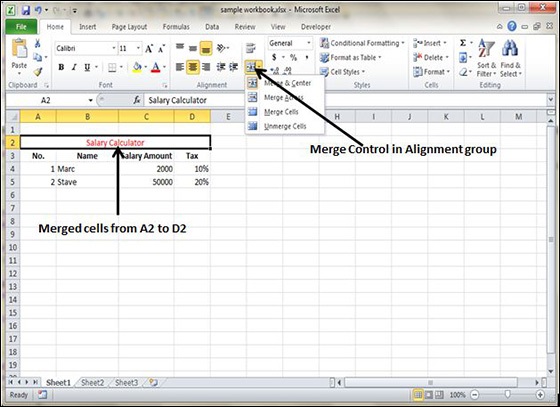
• Choose Alignment tab of the Format Cells dialogue box to merge the cells.

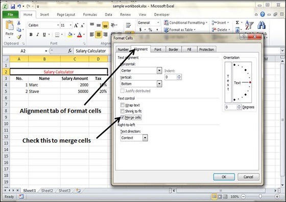
Additional Options

The Home » Alignment group » Merge & Center control contains a drop-down list with these additional options −

• Merge Across − When a multi-row range is selected, this command creates multiple merged cells — one for each row.
• Merge Cells − Merges the selected cells without applying the Center attribute.
• Unmerge Cells − Unmerges the selected cells.

Wrap Text and Shrink to Fit

If the text is too wide to fit the column width but don’t want that text to spill over into adjacent cells, you can use either the Wrap Text option or the Shrink to Fit option to accommodate that text.

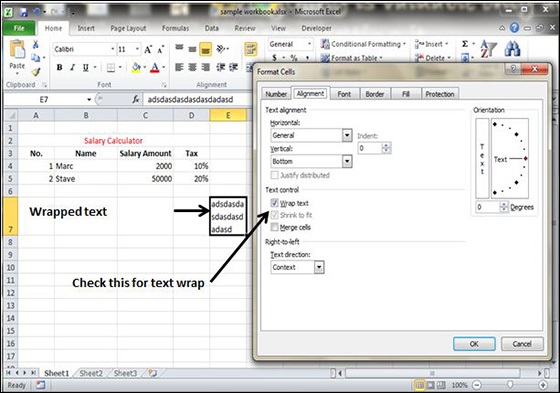
Filters

Filtering data in MS Excel refers to displaying only the rows that meet certain conditions. (The other rows gets hidden.)

Using the store data, if you are interested in seeing data where Shoe Size is 36, then you can set filter to do this. Follow the below mentioned steps to do this.

• Place a cursor on the Header Row.
• Choose Data Tab » Filter to set filter.

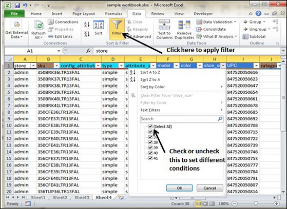
• Click the drop-down arrow in the Area Row Header and remove the check mark from Select All, which unselects everything.
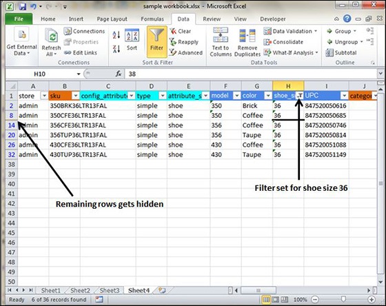
• Then select the check mark for Size 36 which will filter the data and displays data of Shoe Size 36.
• Some of the row numbers are missing; these rows contain the filtered (hidden) data.
• There is drop-down arrow in the Area column now shows a different graphic — an icon that indicates the column is filtered.

Using Multiple Filters

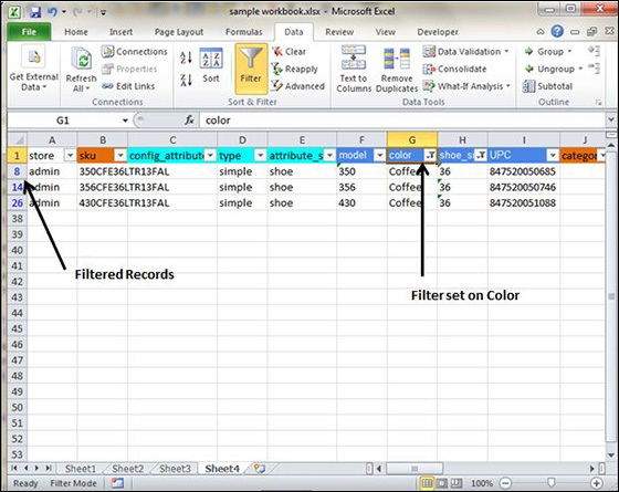
You can filter the records by multiple conditions i.e. by multiple column values. Suppose after size 36 is filtered, you need to have the filter where color is equal to Coffee. After setting filter for Shoe Size, choose Color column and then set filter for color.

Graphic Objects

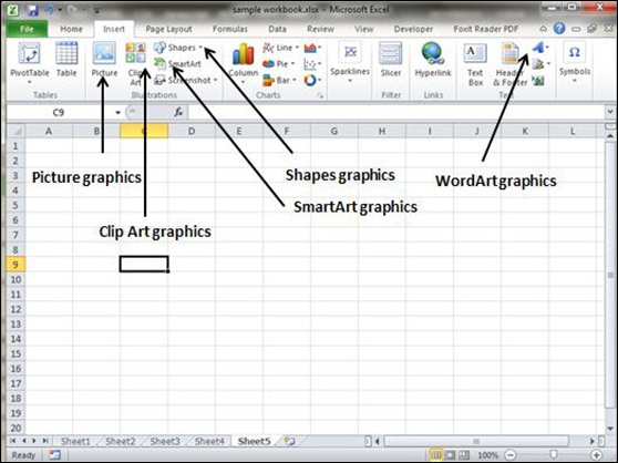
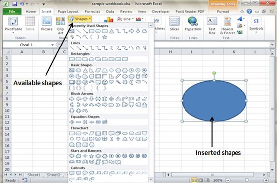
MS Excel supports various types of graphic objects like Shapes gallery, SmartArt, Text Box, and WordArt available on the Insert tab of the Ribbon.Graphics are available in the Insert Tab. See the screenshots below for various available graphics in MS Excel 2010.

Insert Shape

• Choose Insert Tab » Shapes dropdown.
• Select the shape you want to insert. Click on shape to insert it.
• To edit the inserted shape just drag the shape with the mouse. Shape will adjust the shape.

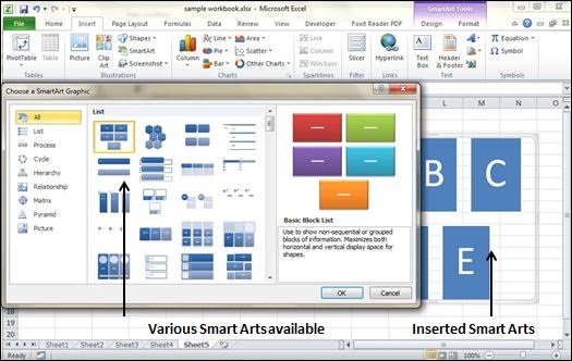
Insert Smart Art

• Choose Insert Tab » SmartArt.
• Clicking SmartArt will open the SmartArt dialogue as shown below in the screen-shot. Choose from the list of available smartArts.
• Click on SmartArt to Insert it in the worksheet.
• Edit the SmartArt as per your need.

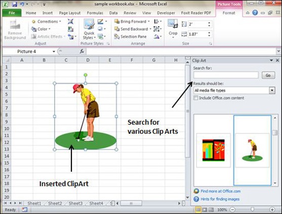
Insert Clip Art

• Choose Insert Tab » Clip Art.
• Clicking Clip Art will open the search box as shown in the below screen-shot. Choose from the list of available Clip Arts.
• Click on Clip Art to Insert it in the worksheet.

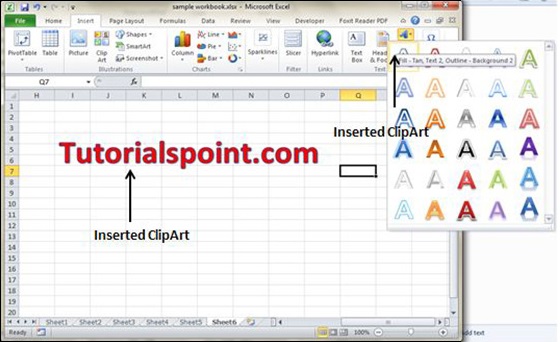
Insert Word Art

• Choose Insert Tab » WordArt.
• Select the style of WordArt, which you like and click it to enter a text in it.